Sentinel-2 satellite data proved to be a reliable source of information regarding the monitoring of Earth features and phenomena’s. With a 10 m geometric resolution is the best optical satellite data available free of charge. The temporal resolution is also performing well, the satellites in the Sentinel-2 constellation provide a revisit time of 5 days. The swath width of Sentinel-2 is 290 km. In comparison, the swath width of LANDSAT 5 TM and LANDSAT 7 ETM+ is 185 km, and the swath width of SPOT-5 is 120 km.
This features makes Sentinel 2 perfect for a wide range of applications.
In this exercise we will try to extract water features from a scene using a simple but effective, data extraction methodology. We will explore the reflectance proprieties of water in the Green and NIR bands, B3 and B8 in the Sentinel 2 case (McFeeters 1996): NDWI (McFeeters) = (Green-NIR) / (Green+NIR).
This NDWI should not be confused with another NDWI (also named Normalized Difference Moisture Index, NDMI), which is derived from the near-infrared (NIR) and shortwave infrared (SWIR) channels (Gao 1996): NDWI (Gao) = (NIR-SWIR) / (NIR+SWIR).
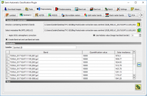
Step 1. Download a Sentinel 2 image using QGIS Semi-Automatic Classification Plugin. Follow the steps presented in the previous tutorial, “Delineate snow using Normalized Difference Snow Index, Sentinel 2 and QGIS” http://www.giscourse.com/delineate-snow-using-normalized-difference-snow-index-sentinel-2-and-qgis/.
Step 2. Preprocess your new downloaded data using QGIS Semi-Automatic Classification Plugin. Set the location folder of the Sentinel-2 bands and the metadata file MSIL1C. This will translate the bands from the default jp2 format to Geotiff format.
2.1 Click Run, set a destination folder and wait until the software finishes the process.
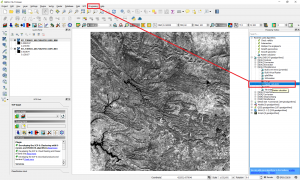
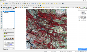
2.2 Open the two bands that we will use for the calculation of the NDWI.
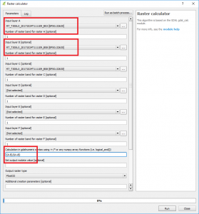
Step 3. Go to Processing > Miscellaneous > Raster Calculator. In this step we will calculate the NDWI.
3.1 Set the Layer A to Band 3 and Layer B to Band 8. In the calculation tab set the formula (A-B)/(A+B). This will perform the operation between the bands and will calculate the NDWI. Set a destination file and click Ok.
3.2 The pixel values should be situated between the values of -1 – 1. To check this, explore the raster histogram.
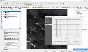
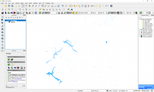
3.3 For a better visualization, we will symbolize the raster. We can observe that the high values are corresponding with the water bodies.

Step 4. Export the results to a vector layer. Use Raster Calculator for masking the water pixels.
4.1 Open the Raster Calculator, following the instructions from Step 3. For Input Layer A set the NDWI calculated. For the calculation formula use A>0. This will create a mask for all the water pixels (with positive value).
4.2 This will create a new mask with 0 and 1 values. Go to Layer Proprieties and set the values Min to 0 and Max to 1.

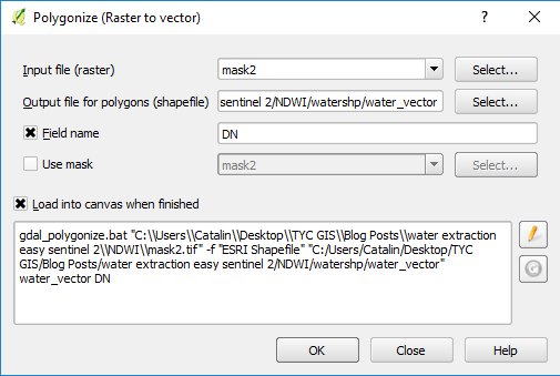
4.3 Go to Raster > Conversions > Translate > Raster to Vector
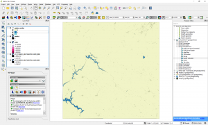
4.4 Symbolize the new vector layer for a better visualization
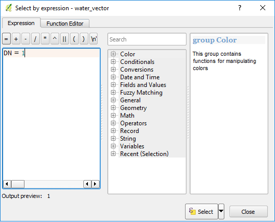
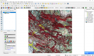
4.5 Export only the water areas. Go to Open Table of Attribute > Select by Expression and write DN = 1.
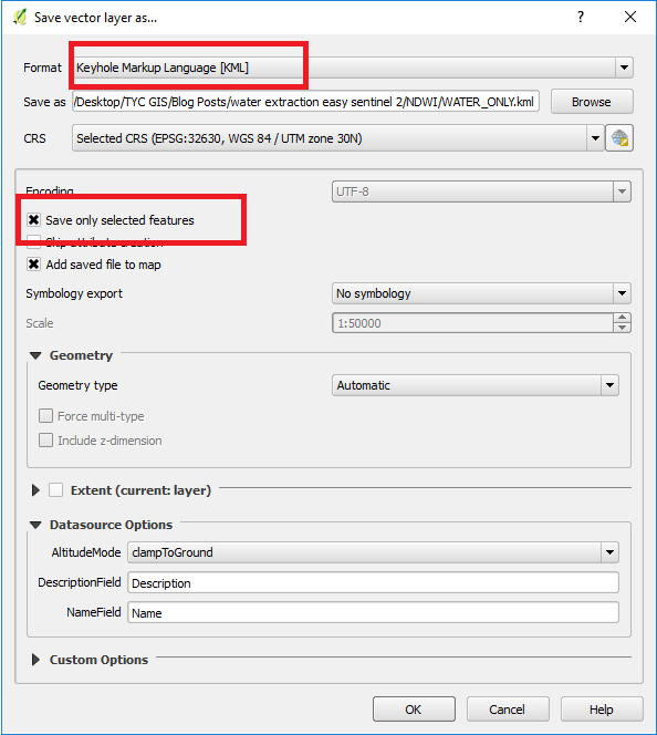
4.6 The water areas will be selected. Next step will consist in exporting the water areas to a separate vector layer KML format. Go to Layers Panel > Right Click on the vector layer and go to Save as. In the menu that will pop up select the format KML (Keyhole Markup Language), the destination file and do not forget to check the Save only selected features box.
4.7 Your results should look like this
Quality training taught by professionals
RECOMMENDED COURSE


Thank you! It was a great help.