Over the last decades, the world of free and open source geo-spatial data and software, has experienced a rapid growth. The concept gained value among professionals from different fields of work, due to its availability and interdisciplinarity. Mapping and understanding the features of the earth became easier.
Natural disasters like floods are happening worldwide. Due to their negative impact on different social, economic and environmental aspects, the need to monitor and map these phenomena has increased. Assessment of flooded areas can be done by using open source remote sensing images acquired by optical and radar sensors.
Flood mapping with radar images
The optimal solution for monitoring and mapping flooded areas is the use of radar data (SAR). Considering their capacity to penetrate clouds, radar sensors can acquire data under any weather conditions during day and night. However, Radar data is normally expensive and unavailable for public use.
The demand for closer to near real time information, free data, higher spatial resolution as well as fast assessment of the damages has forced the European Union and the European Space Agency to provide open access to the new missions of the Copernicus earth observation program (ESA, 2015, Copernicus Final Reports, http://www.esa.int/Our_Activities/Observing_ the_Earth/Copernicus/Final_reports).
The development of ESA Sentinel-1 missions (radar with 10 m spatial resolution and a revision time of 5 days in constellation mode), set a new milestone in the flood assessment and risk mitigation.
Ebro River Flood – February/March 2015
During February/March 2015 an important flood affected middle course of Ebro River. The event lasted 17 days from February 23 to March 11 and registered a maximum flow near the city of Zaragoza in the early morning of March 2nd.
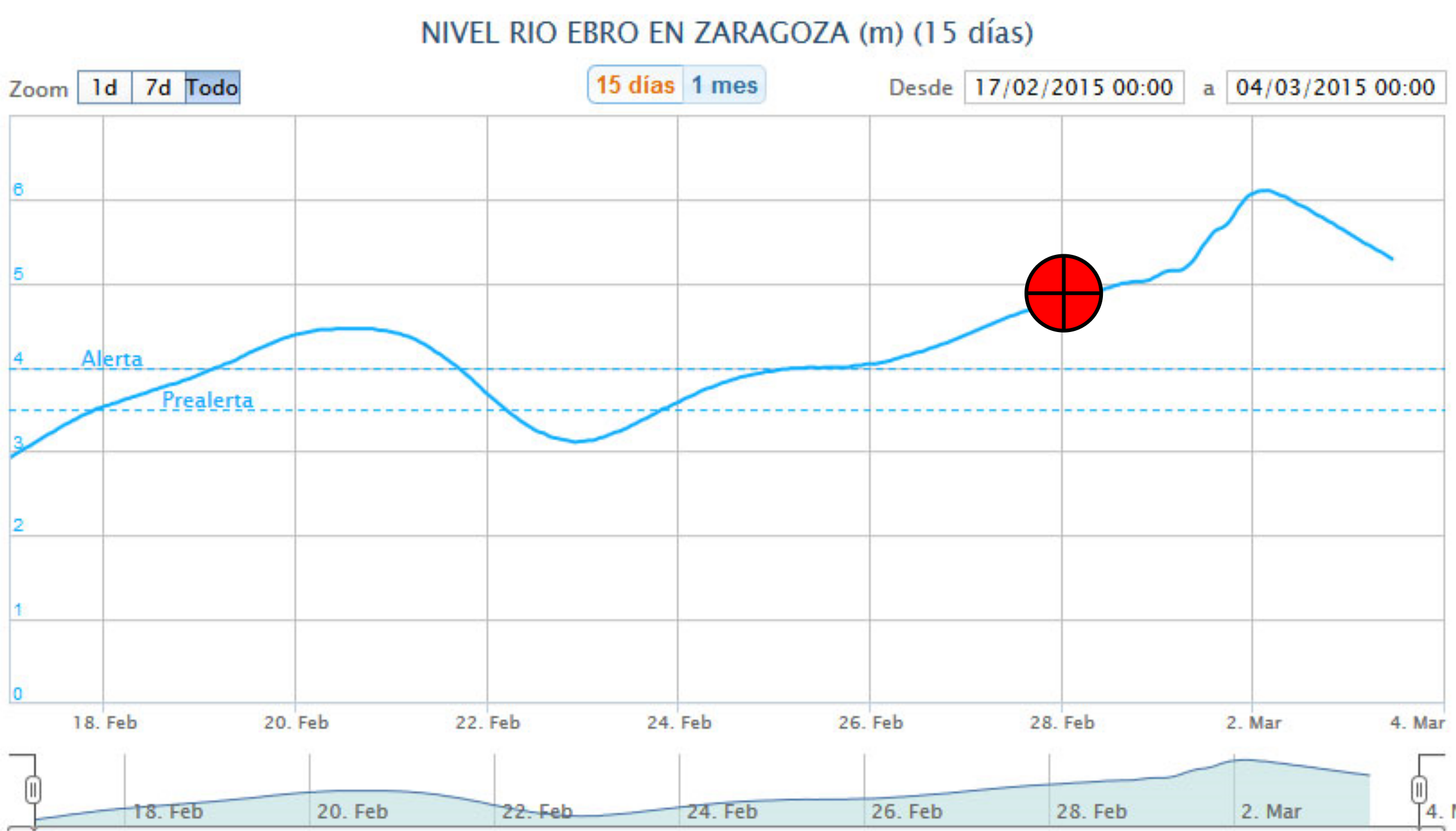
Figure 1: Ebro River Levels at Zaragoza since 18 February 2015. Image source: Confederación Hidrográfica del Ebro
Example of flood extend delineation using SNAP and Sentinel-1. Case study: Ebro River
Step 1: DATA PREPARATION
In this tutorial, Level-1 Ground Range Detected (GRD) Sentinel-1 C-band data, collected in IW mode (Interferometric Wide) was used. This mode allows image acquisition over a 250 km swath width with a geometric resolution of 10 m (5x20m).
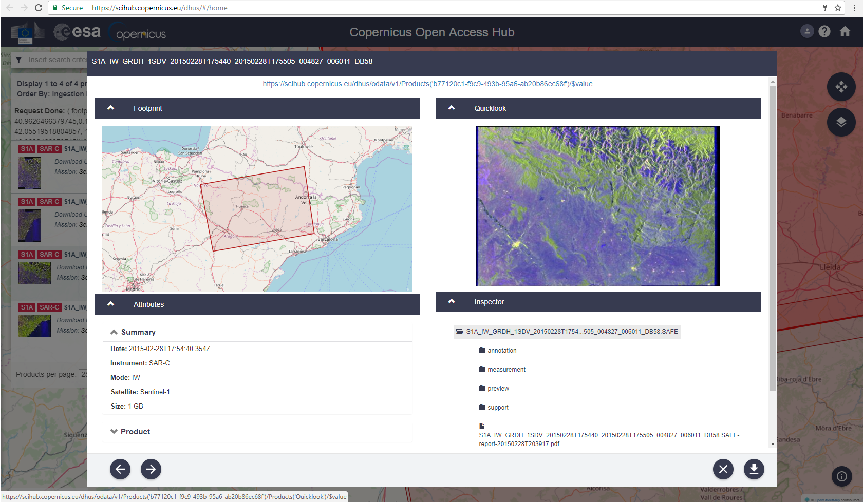
1.1 Download Level-1 Ground Range Detected (GRD) Sentinel-1 C-band data from Copernicus Open Access Hub (https://scihub.copernicus.eu).
A Level-1 Ground Range Detected (GRD) Sentinel-1 image dated from February 28, 2015 was downloaded. The image captures the flood in its middle stage according to the graph above.
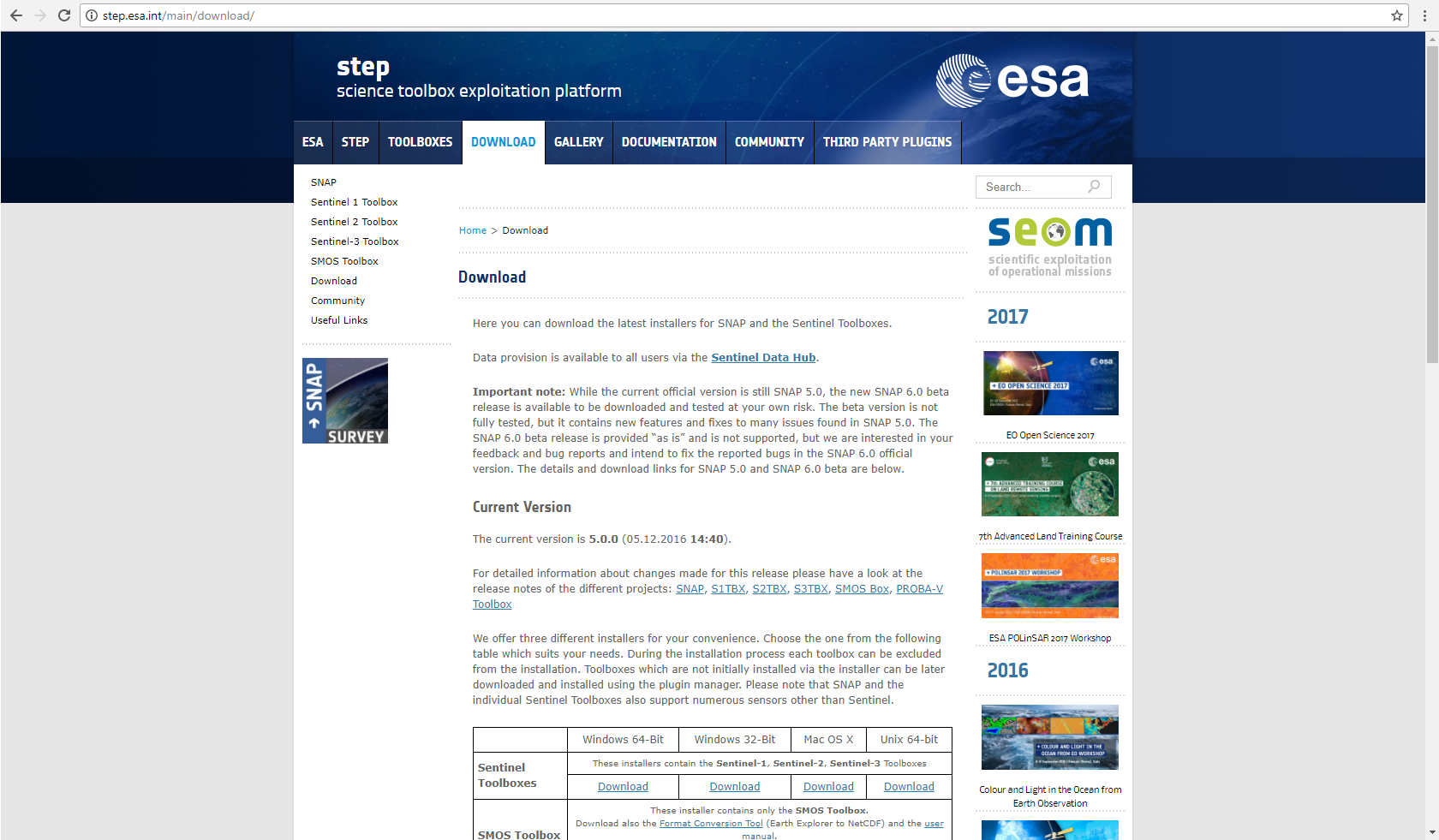
1.2 Download SNAP and Sentinel Toolboxes from http://step.esa.int/main/download/.
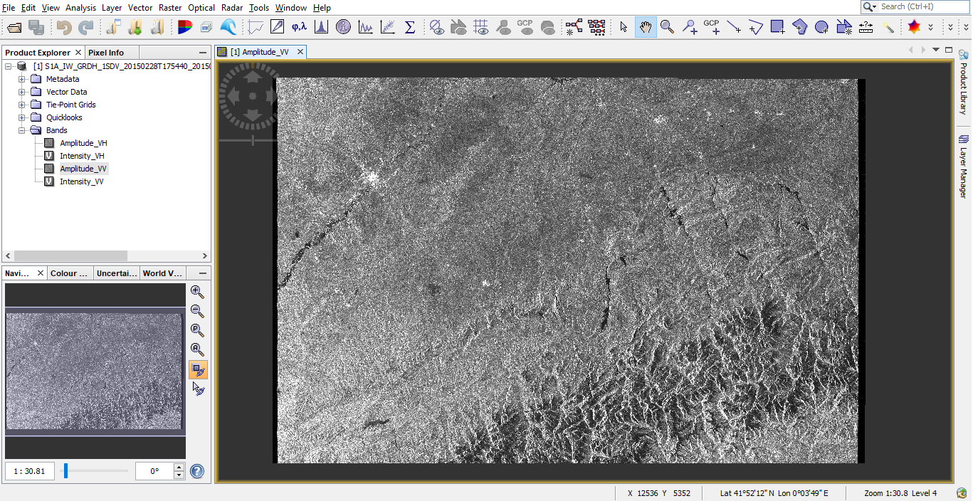
1.3 Open product in SNAP: File > Open Product
After the product is opened, the Product Explorer on the left, will show relevant information about it: Metadata, Bands (acquired in dual polarization HH+HV or VV+VH), etc.
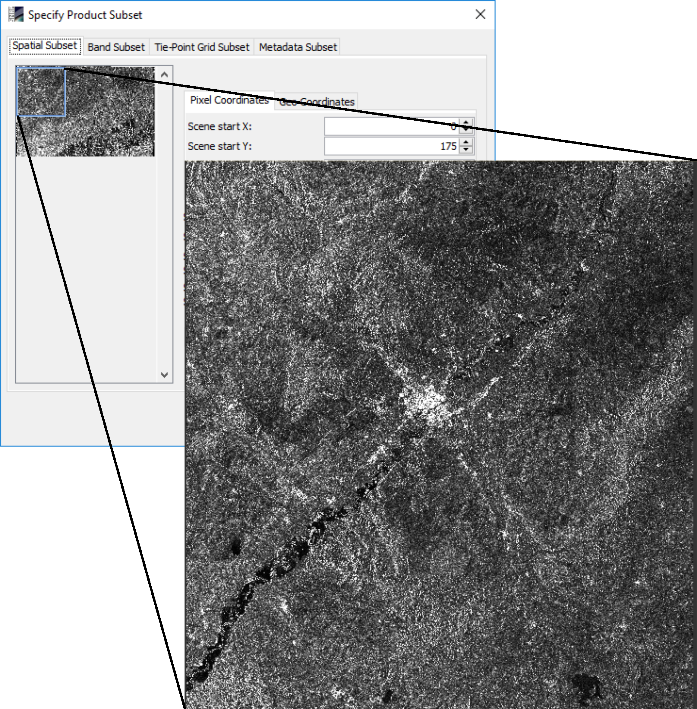
1.4 Create a subset focused on the interested area: Raster > Subset
Step 2: PRE-PROCESSING – CALIBRATION AND SPECKLE FILTERING
SAR calibration provide imagery in which the pixel values can be related to the radar backscatter of the scene. This step transforms the pixel values from the digital value recorded by the sensor into values of backscatter coefficient.
2.1 Radar > Radiometric > Calibrate > Processing Parameters and select your preferred polarization.
The Calibration tool will create a new product with calibrated values of the backscatter coefficient. The next step consists in the removal of the speckle noise which is a very important step in the process of obtaining high-quality radar images.
2.2 Select Radar > Speckle Filtering > Single Product Speckle Filter > Processing Parameters and select your preferred filter. Many filters exist, but for this tutorial we used the Lee filter, with a window size of 5×5 pixels. This means that within a sliding window of 5 pixels high by 5 pixels wide, a pixel is equal to the local mean and variance of all pixels within the moving kernel.
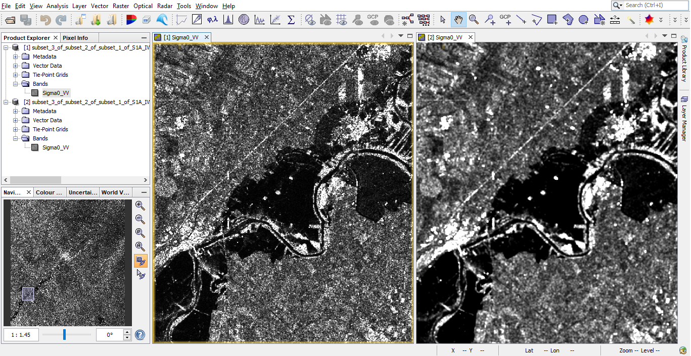
Sample of the product before and after Speckle Filtering.
Step 3: DETERMINATION OF AREAS COVERED BY WATER
3.1 Setting a threshold to the calibrated backscatter coefficient
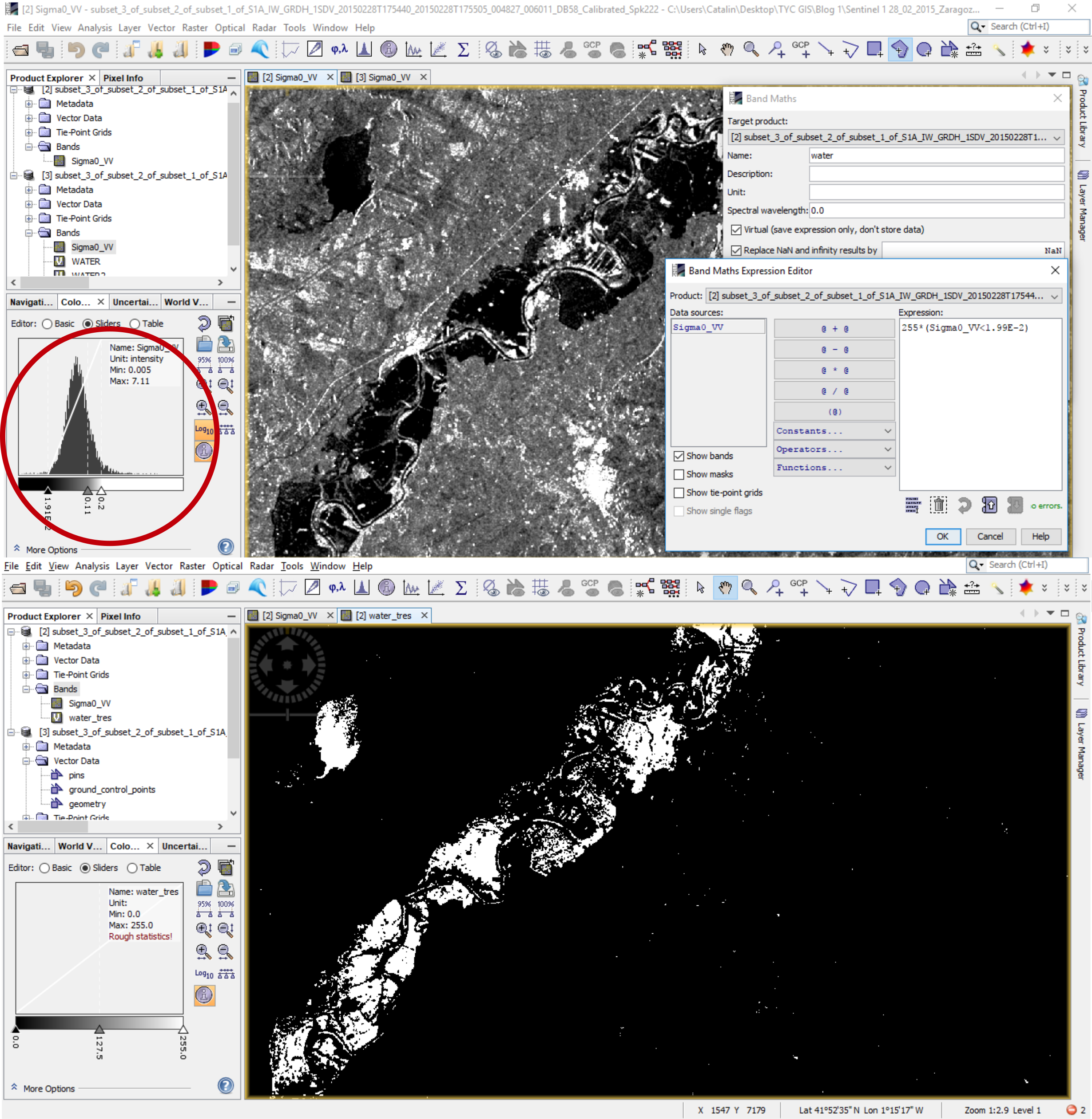
Using the histogram of the calibrated backscatter coefficient, and applying a threshold, the water pixels can be separated from the non-water pixels. Low values on histogram coincide with the water class. Different thresholds must be chosen in order to get the best representation for the water areas.
The thresholds can be set using: Raster > Band Math > Edit Expression
3.2 Using supervised classification method – Maximum Likelihood
In supervised classification the user supervises the pixel classification. The user specifies the various pixel values that should be associated with each class. This is done by choosing representative sample sites of known land cover types. This representative samples are known as training sites or areas. The software then uses these training sites and applies them to the entire image.
There are different classification algorithms. For this exercise we used the Maximum Likelihood algorithm. The algorithm assumes that the statistics for each class in each band are normally distributed and calculates the probability that a given pixel belongs to a specific class. Each pixel is assigned to the class that has the highest probability.
To classify the image in two classes (Water and Non-Water), specific training areas corresponding to each class were digitize. To perform this operation use: Vector > New Vector Data Container (create two vectors Water and Non Water) and with Polygon Drawing Tool select the best representative areas for each class as shown in the image below.
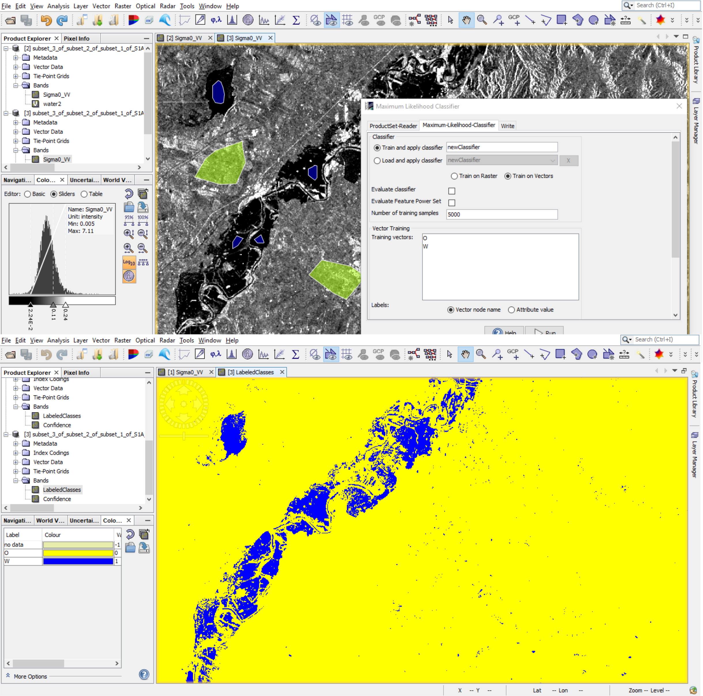
To perform the classification, follow: Raster > Classification > Supervised Classification. The results should look like in the image above.
Step 4: POST-PROCESSING – GEOMETRIC CORRECTION
The image is in the acquisition geometry of the sensor. The pixels do not have geographical coordinates. The geometric corrections will project the image in the preferred geometry. In our case ED50 UTM zone 30N. Radar > Geometric > Terrain Correction > Range Doppler Terrain Correction. You must be connected to the internet, the Digital Elevation Model SRTM will download automatically, if there is no Internet connection, set External DEM and chose your already downloaded DEM from the menu Digital Elevation Model. Leave the Map projection to its default WGS84 (DD) and unable the parameter Mask out areas without elevation, then run the process. This will create a new image in a Geographic Coordinate System Lat/Lon (WGS84) projection.
Projected Coordinate System ED50 UTM zone 30N can be obtained by following the following steps: Raster > Geometric Operations > Reprojection

The difference between a Geographic Coordinate System (WGS84) based on a spheroid and a Projected Cordinate System based on a 2D plan (ED50 UTM zone 30N).
Step 5: EXPORT DATA TO PREFERRED FORMAT
The new obtained data can be exported in different formats to match other software requirements. For Google Earth visualization select: File > Export > Other > View as Google Earth KML KMZ.
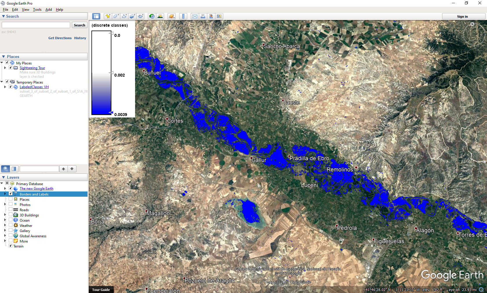
State of the flood on February 28, 2015.
Quality training taught by professionals


Hi . This is khalid from afghanistan . I would like to join the class .how it’s possible
Hello! If interested please send an e-mail to training@tycgis.com.
Thank you!
Hello. I’m Joaquim Egas from Mozambique. I interested to join to the class.
Hello!
If interested please send an e-mail to training@tycgis.com.
Thank you!
Hi,
I would like to join this course.Please let me know the details of the course.
Thanks.
Hello!
If interested please send an e-mail to training@tycgis.com.
Thank you!